
LKAJJFLKDJF


LKAJJFLKDJF
Last edited by DocAElstein; 02-16-2024 at 12:02 AM.
Some notes from a deleted post answering/replying to a snb troll here : https://eileenslounge.com/viewtopic....303506#p303506
( chttps://excelfox.com/forum/showthread.php/2345-Appendix-Thread-(-Codes-for-other-Threads-HTML-Tables-etc-)?p=18405&viewfull=1#post18405
)
Some Notes Comparison in support of this forum post.
https://eileenslounge.com/viewtopic....303506#p303506
Some notes to compare / consider this: https://eileenslounge.com/viewtopic....303487#p303487So,
Selection.Value = Evaluate("=IF({1},TRIM(SUBSTITUTE(" & Selection.Address & ",CHAR(160),CHAR(32))))")
, and this
Originally Posted by snb post_id=303506 time=1674152398 user_id=5598
… not sure what is to be got from that. Could be a typical snb Troll , or something useful. snb’s posts are usually some combination of the two. But I have a bit of time, this time around, so my take on it,
………………..
Wot are we looking at / comparing / considering….
This was my basic one liner
Let Selection.Value = Evaluate("=IF({1},TRIM(SUBSTITUTE(" & Selection.Address & ",CHAR(160),CHAR(32))))")That includes the usual trick of
IF({1},__The main bit __ )
That trick is to get array values out when they often don’t , mostly in earlier Excel versions, 2013 and lower. So the main bit is
Let Selection.Value = Evaluate("=TRIM(SUBSTITUTE(" & Selection.Address & ",CHAR(160),CHAR(32)))")In fact that main bit is most likely all you need for Excel 2016 +
So, I am comparing that/ considering the “Evaluate” alternative from snb
Selection.Name = "snb"
[snb].Replace Chr(160), " "
[snb] = [index(trim(snb),)]
_.________________________
These two lines:, (or part thereof)
Selection.Name = "snb"I have seen this from you snb, in a few places, ( example, https://excelfox.com/forum/showthrea...ull=1#post9714 )
[snb]
It is an interesting way to make some thing dynamic that you might normally need to hard code:
To explain:
We can do an Evaluate in a couple of ways
_ The way I like to do it: __ Evaluate(“___“)
and
_ a shorthand way _________ [___]
The advantage of the first over the second way is that because the syntax insist you build the thing, ___ , in a string, that string can include variables, making a solution dynamic.
The second way would usually need to be hard coded. In this example it is hardcode, but hard coded to the name of a range, so in a round about way its made dynamic.
It seems a bit of a red herring here, we can replace
____ Selection.Name = "snb"
____ [snb].
with
____ Selection.
So unless I missed something we have gained nothing , just confused and obfuscated there.
_._______________________________
.Replace
.Replace Chr(160), " "
I confess I have not used much the VBA Range.Replace method ( https://learn.microsoft.com/en-us/of....range.replace ) much, but it seems to have some similar arguments to the VBA .Find method.
Used here I see no advantages over the Excel SUBSTITUTE. It has the disadvantage here that it introduces another line. Approximately, in effect it has done like replaced one line,
__ TRIM(SUBSTITUTE(" & Selection.Address & ",CHAR(160),CHAR(32)))
, with 2 lines
__ X = SUBSTITUTE(" & Selection.Address & ",CHAR(160),CHAR(32))
__ TRIM(X)
_.____________________________
This line: _ [snb] = [index(trim(snb),)]
This is approximately the second of the 2 code lines above. It’s this one
__ Selection.Value = Evaluate("=TRIM(X)")
_.__________________________________
Some other stuff/ observations / comments :
A couple of things
_(i) " "
_(ii) Index(___ , )
These two things are couple of things written in a slightly different way
_(i) " "
That is a simple text space, - in Excel can be written as CHAR(32) and in VBA as Chr(32)
_(ii) Index(___ , )
For Office versions 2016 and lower versions , some things annoyingly do not return us an array of results. Often the results are there., somewhere, but they annoyingly are not given. ( There seems to be a parallel in the way it works to how things in a spreadsheet work or don’t, depending on whether you enter normally or do the so called CSE thing).
There is no documentation on this, but people have found empirically that some tricks used in Evaluate(" ") get us the array of results we want on the occasions that they annoyingly do not otherwise appear. One that has been used for many years was
INDEX(___ , ) , where ___ is the thing you want an array of results from, and you suspect it has, but is annoyingly not giving you.
A few years back I** stumbled on this alternative, which usually seems to do the same
IF({1},___)
( ** It is possible that someone else noticed that before I did. I never saw any examples yet, but I claim no “ownership” of it )
_.________________________________
Summary ( of snb’s post )So its close to my solution, in a less efficient way and in an obscure, obfuscated form.
Not really an alternative solution.
Probably more trouble than its worth this time around. Bit of a Troll really, Lol
Interesting only if you have a lot of free time and are bored.
Alan
Last edited by DocAElstein; 02-16-2024 at 01:10 AM.

Hi Alan... Thank you so much , thank you for your explanation as this has helped be understand more of what the code does... sometime this is more important than the solution itself.
Keep up the good work.
Thanks again
Paul
Last edited by DocAElstein; 02-16-2024 at 12:07 AM. Reason: Took out the long quote in reply
You're welcome , Paul , thanks for the feed
Last edited by DocAElstein; 02-16-2024 at 12:02 AM.
This is post https://www.excelfox.com/forum/showt...ll=1#post18640
https://www.excelfox.com/forum/showt...ge18#post18640
Building and breaking ( up ) some formulas in cells
Some notes, coding breakdown to go with this post
https://eileenslounge.com/viewtopic....314208#p314208
For consistency / better comparison of offerings, we will use the same test data that I have used in that Thread ( https://eileenslounge.com/viewtopic....314200#p314200 ) a few times , that is a few rows where I have numbers in
https://i.postimg.cc/NjzZxy0C/Test-d...n-column-D.jpg
5 rows of numbers to be summed.JPG
_____ Workbook: Leading Apostrophe, Text in cells.xls ( Using Excel 2007 32 bit )
Worksheet: Tabelle1
Row\Col A B C D E 1 10 11 20 2 11 12 21 3 12 13 22 4 13 14 23 5 14 15 24 6
There are two snb offerings, that I will look at and ramble off in tangents probably as well, Lol
, and we will look at the first one in this post, which is very easy and basic if you sanitise the snb obfuscation as I do in this first TLDR explanation
, and we will look at the second one in the next post ( https://www.excelfox.com/forum/showt...ll=1#post18641 , https://www.excelfox.com/forum/showt...ge18#post18641 ) , which is a more typical snb one liner coding offering, but still is a bit obfuscated on top of that, or so I thought…
S0… This one first:
The TLDRCode:Sub M_snb() ' https://eileenslounge.com/viewtopic.php?p=314208#p314208 With Cells(1).CurrentRegion .Offset(, .Columns.Count).Resize(, 1) = "=A1+B1+C1" End With End Sub
There is not much to say about this offering. - It sort of, puts the formula string, "=A1+B1+C1" down the column range D1:D5 That formula string needs some further explanation as below, but to avoid unnecessary obfuscation confusion, lets first say that this bit,
Cells(1).CurrentRegion.Offset(, .Columns.Count).Resize(, 1), is just an obfuscated way to say Range("D1:D5")
So that coding can be written in this simpler way, in one code line
( The small functionality difference, to Range("D1:D5") is that the last row is got if you don’t know it, (assuming your test range is isolated by at least one free columns so that Cells(1).CurrentRegion will work). It makes the coding debatably compact or obfuscated, personally I would say obfuscated if the thing is supposed to be demonstrating a way to do something, JIMHO. )Code:Sub PutA1andB1andC1InColumnD() ' Range("D1:D5") = "=A1+B1+C1" ' LHS see https://www.excelfox.com/forum/showthread.php/2918-Right-Hand-Side-Range-Range-Value-values-Range-Range-Value-only-sometimes-Range-Range-Value-Anomaly?p=23192&viewfull=1#post23192 https://www.excelfox.com/forum/showthread.php/2914-Tests-and-Notes-on-Range-objects-in-Excel-Cell?p=22099&viewfull=1#post22099 RHS see https://teylyn.com/2017/03/21/dollarsigns/#comment-191 End Sub
_.__________________________
Some more detailed explanations of the basic formula of this type:
Range("D1:D5") = "=A1+B1+C1"
LHS , Range("D1:D5") =
Most of us think we know what that is about, we are close enough with our thinking on that
( Here are some recent notes on what the left hand side (LHS) of the single code line is all about , most of us already think we know all about, we are not far off, but I think, for now, I have it better sussed than anyone,,
https://www.excelfox.com/forum/showt...ll=1#post23192
https://www.excelfox.com/forum/showt...ll=1#post22099 )
RHS , = "=A1+B1+C1"
The right hand side, ( RHS ), could do with being considered and explained a bit better than it usually is ….
Two similar main topics are required in this explanation
_1 When we tell / ask / give excel to do something, we often do that in a singular, or similarly simplified way that is more humanly conveniently for us. The original idea of Excel is to reduce our tedious work, in particular tedious repetitive work. As part of this, a common practice is that we ask something to be done across a range of cells, that is the LHS and on the RHS in the most simplified explanation, we give it the information for a single cell, conventionally top left of the range. Depending on exactly what information we give, ( that is _2 ) , Excel will apply what it thinks we want to all the cells in the range. In fact, we will see that Excel simply puts exactly the same thing in every cell!!!
So that’s topic _1 one covered
_2 What we give
We are giving a single cell reference. Excel has two conventions , or "languages" that it understands when giving and receiving cell references. We are using the so called "A 1 column letter and row number notation" ( The other is the so called "R C row and column number notation”, which we will only consider briefly )
Those two conventions differ mainly only in the way they are physically shown. Both conventions have within them two basic concepts/ things that we can use. One is simple: An absolute grid or co ordinate or x y reference to a single cell. ( Some thing looking like this $A$1 $Y$34 etc. in the "A 1 column letter and row number notation" way of showing, or like R4C8 R1C1 etc in the "R C row and column number notation"). If we give that fixed absolute grid reference type of thing, then Excel very easily sees that across the range given on the LHS, the same cells will always be referenced to regardless of which cells are used for the final output that we are looking for. So for a simple formula we would always get the same result in every output cell.
In other words, in simple terms referring to our actual example, the use of "=$A$1+$B$1+$C$1" on the RHS will result in the same sum formula of the first row will be done in every cell in the column D range, D1:D5
That is simple, no great intelligence, Human of artificial to do that.
We are not concerned with that here.
The second way/ concept that we are concerned with here, is the concept that helps Excel to give us what we want, if we want something slightly less simple. Because in everyday requirements this slightly less simple way is more often what we want, then the way we see or give Excel these cell references most often is in this apparent simpler A1, Y34, etc. way, - this apparent simplicity unfortunately disguising that it is actually indicating the more advanced of the two possibilities. It is not a simple x y grid type reference as it may appear to be.
Now, _1 told us that what we give as a single formula in the RHS will be taken as best Excel can to be put in all the cells in the range we give on the LHS. In fact although it’s not obvious, it simply puts exactly the same thing in each cell. It gives not an absolute grid or co ordinate or x y reference as it might be assumed, but rather a fixed vector or relative cell reference. So exactly the same thing is in fact put in the cell, it just does not look like it
A slightly more detailed explanation of these last concepts are given here: https://www.excelfox.com/forum/showt...ll=1#post24006
We cannot so easily see in the "A 1 column letter and row number notation" style "language" the underlying formula that Excel puts in the cells D1:D5. This typically regarded meaningful list of the actual formulas in the is actually a bit misleading
=A1+B1+C1
=A2+B2+C2
=A3+B3+C3
=A4+B4+C4
=A5+B5+C5
( For convenience, use these flipping two code lines that snb gave, https://eileenslounge.com/viewtopic....256ef4#p314221 , to get a formula spreadsheet )
It is slightly easier if we look at the exact same formulas, but just shown in the other way of showing them. Which is no change to the actual formulas, they are exactly the same formulas, just written in an alternative form but which means the exactly same thing
=RC[-3]+RC[-2]+RC[-1]
=RC[-3]+RC[-2]+RC[-1]
=RC[-3]+RC[-2]+RC[-1]
=RC[-3]+RC[-2]+RC[-1]
=RC[-3]+RC[-2]+RC[-1]
Excel has actually simplified that for us, the more explicit form of that formula used in every cell would be
=R[0]C[-3]+R[0]C[-2]+R[0]C[-1]
( Change your options to get the different convention of "R C row and column number notation”. Example in Excel 2007
https://i.postimg.cc/RZ9NHdnY/Excel-2007-Options.jpg https://i.postimg.cc/X79rqmXF/Excel-...e-language.jpg )
What that is telling us is that we have something like a fixed vector or fixed offsets to take us to the cell from which to get the values, specifically
0 row offset , in other words the same row
and
either 1 , 2, or 3 columns offset to the left. (The general convention in Excel is that left to right is positive and visa versa , so to the left is negative)
The "A 1 column letter and row number notation" makes it look like we put a different formula in each cell, but we don’t. Excel is just sowing the same fixed vector in a different way: by showing us the cell at the one end of the vector when the other end is put in the cell where the formula is. That is just the way Excel was designed: in the "A 1 column letter and row number notation" it gives a direct indication of the cell used. This way of showing things can explain the idea of dragging a formula down, - if a formula is written in the relative ( fixed vector ) way of the "A 1 column letter and row number notation", then dragged down, it will appear that Excel is adjusting the formula to reference the appropriate cells, but its not really. It’s really dragging down exactly the same thing which then is shown in a way that will make it appear different in different cells.
That’s about it
Conclusion
In the range D1:D5 the same formula is put in. They all get the 3 values to sum from the same row and either 1, 2 , 3 cells to the left. Think of it as three horizontal pipes of different lengths, the second twice as long as the third 3 times as long as the first
When using this way it is important to use the relative ( fixed vector ) way of the "A 1 column letter and row number notation", since if we used the fixed spreadsheet coordinate way of the "A 1 column letter and row number notation", like =$A$2+$B$2+$C$2 , then it would not work as we want it to: It would in fact, in every cell in the range D1:D5, sum the values of the 3 column in the first row, Just as dragging that formula down would give us
=$A$1+$B$1+$C$1
=$A$1+$B$1+$C$1
=$A$1+$B$1+$C$1
=$A$1+$B$1+$C$1
=$A$1+$B$1+$C$1
( Ref https://teylyn.com/2017/03/21/dollarsigns/#comment-191
Windows display formulas https://eileenslounge.com/viewtopic....314221#p314221
Excel option R C or A 1 type display https://i.postimg.cc/RZ9NHdnY/Excel-2007-Options.jpg https://i.postimg.cc/X79rqmXF/Excel-...e-language.jpg
https://www.excelfox.com/forum/showt...ll=1#post24006 )
Last edited by DocAElstein; 02-22-2024 at 01:52 PM.
This is post https://www.excelfox.com/forum/showt...ll=1#post18641
https://www.excelfox.com/forum/showt...ge18#post18641
From the last post we know the LHS is justCode:Sub M_snb__() ' https://eileenslounge.com/viewtopic.php?p=314208#p314208 With Cells(1).CurrentRegion .Offset(, .Columns.Count).Resize(, 1) = Evaluate(Replace("index(A1:A~+B1:B~+C1:C~", "~", .Rows.Count) & ",)") End With End Sub
Range("D1:D5") =
As for the RHS, this turned out to be much less signifiucant and more in the directon of a troll / obfuscation than I thought.
At first glance perhaps a typical quite clever compact coding typical of some of snb’s, but after a close inspection it looks like less so – as the OP, ErikJan, was a obviously in a bit of stress at the time, then posting stuff like this to him was perhaps a bit unkind, a typical Troll by any standards.
Working a bit backwards, as in the specific example it helps clarify things a bit quicker:
Consider these two things,
Index( ___ , )
If({1},____ )
The stuff in black is a trick, usually done finally when we find that a CSE type spreadsheet formula, put inside Evaluate(" ") in VBA does not give us the same multiple results as in the spreadsheet. Specifically, annoyingly sometimes, it give us just one answer, corresponding usually to something like the first cell result.
Or saying the same thing a bit differently: in those two things , to a first approximation , the purple bit is the main thing we are considering here, or the main solution type which I am trying to explain
This solution type is what I call, and what I know more about than anyone else on this planet, even snb in the meantime, is the so called, or Alan called, Evaluate("____") Range type solution. These solutions work in a similar way to the so called "array formulas" or "CSE (type 2) formulas" in an excel spreadsheet. But for earlier versions of Excel they annoyingly don’t always work and give us just one answer, corresponding usually to something like the first cell result. We talk then about tricks, "coercing", and the such to get them to give us an array of values, in other words all the values. Those extra bits in black, INDEX( ___ , ) or IF( {1}, ___ ) , are a bodge / trick to make these things work as they mostly do. They only occasionally are needed, and when they are needed they will be needed in all Excel versions before 2016. If you find that they are not needed in any version of Excel before 2016, then they never will be
So they are not always needed, and in fact, it turns out, they are not needed at all in this case, so we can forget all about them here, and so changing this
= Evaluate(Replace(" index(A1:A~+B1:B~+C1:C~", "~", .Rows.Count) & " ,)")
, to this
= Evaluate(Replace("A1:A~+B1:B~+C1:C~", "~", .Rows.Count) & "")
, will have no effect.
Once we have that out of the way, we can see perhaps that the VBA Replace is giving us in effect the last row, (5 , if we use the same examples test range I have been considering most of the time).
To elaborate a bit in words, in case it’s not obvious what we are doing with the replace. The VBA Evaluate used in the Evaluate(" ") specifically takes a string rather than just the same text you would put in a cell
in other words with a simple example, we would need this
Evaluate("=1+1")
rather than
Evaluate(=1+1) )
There is at least one very good reason for , or good outcome of, that. The reason being is that at the end of the day a string wants to be seen there. But importantly, how that string comes about is of no interest to Evaluate( ). First the string will be got, **if it can be, ( **assuming no syntax error , etc. )
In our case we have this thing, which is a VBA thing,
Replace("A1:A~+B1:B~+C1:C~", "~", .Rows.Count)
Now, Rows.Count is another VBA thing and will first be done and will return 5 for the test range I have mostly been using, so we have, ( still in VBA things being done initially )
Replace("A1:A~+B1:B~+C1:C~", "~", 5)
So the way the VBA Replace works in this form is that in the string "A1:A~+B1:B~+C1:C~" , the ~ is replaced with 5 retuning us this final string which evaluate works on
"A1:A5+B1:B5+C1:C5"
So at the end of the day we have this,
Range("D1:D5") = Evaluate("A1:A5 + B1:B5 + C1:C5")
This is very similar to doing manually, in the spreadsheet.these 3 steps
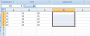
_ step 1 - select the entire range D1:D5, that would be something equivalent to the VBA code line LHS, defining the range to put stuff in, or to apply the RHS to.
https://i.postimg.cc/X7gctgvH/Select-Range-D1-D5.jpg
The next two steps are doing something similar to the RHS of the VBA code line, - in simplest terms, the this bit inside the Evaluate("____") is approximately like what is in a cell, in other words Evaluate here evaluates stuff as it would be evaluated in a cell. (When multiple ranges are in this bit , then it is something like doing the so called "array formulas", except that we do not have the necessity to do the CSE related things as they are necessary to allow the spreadsheet to adjust to receiving and presenting more that one result, whereas the Evaluate returns type Variant, allowing amongst other things an array to be returned. )
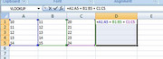
_ step 2 type in =A1:A5 + B1:B5 + C1:C5 ( you might want to click in the formula bar and type it in there, just to be sure that you are not just typing it in one cell, which you don’t want to be doing.
https://i.postimg.cc/WbVw9ysq/write-...1-B5-C1-C5.jpg
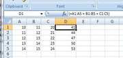
_ step 3 Now you do that so called "array formula CSE type entry" , and you should see all the results as expected.
https://i.postimg.cc/sf7J4zCR/CSE-2-entry.jpg
In this particular example our Evaluate("A1:A5 + B1:B5 + C1:C5") inside VBA will give us that array of values
{41
44;
47;
50;
53}
VBA allows us to apply a field of values ( an array ) to a range in one go, which is what we do.
Range("D1:D5") = Evaluate("A1:A5 + B1:B5 + C1:C5")
Last edited by DocAElstein; 02-22-2024 at 05:44 PM.
ashchackhch
Last edited by DocAElstein; 02-16-2024 at 12:00 AM.
hhhdhhc
Last edited by DocAElstein; 02-15-2024 at 11:59 PM.
asdjccsdjhchcsdhc
Last edited by DocAElstein; 02-15-2024 at 11:58 PM.
fhqhfhfh
Last edited by DocAElstein; 02-15-2024 at 11:58 PM.
 Posting Permissions

 Reply With Quote
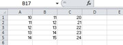
Bookmarks