Code:
Option Explicit
Sub PartsIP() ' ***** Select Top left of range to be used in worksheet AllIPs
Rem 0 Worksheets and data range info
Dim wsAllIPs As Worksheet, WsSts As Worksheet
Set wsAllIPs = ThisWorkbook.Worksheets("AllIPs"): Set WsSts = Me ' ThisWorkbook.Worksheets("StatsIP")
Dim TLa As Range, Lra As Long, TLs As Range, Lcs As Long, Lrs As Long
Set TLa = Selection ' ***** Select Top left of range to be used in worksheet AllIPs
Let Lra = wsAllIPs.Cells.Item(wsAllIPs.Rows.Count, Selection.Column).End(xlUp).Row
Let Lcs = WsSts.Cells.Item(1, WsSts.Columns.Count).End(xlToLeft).Column
Dim NxtClm As Long: Let NxtClm = Lcs + 2 ' Top left of where the new column pair will go
Rem 1 Copy data to Stats worksheet, ( twice )
wsAllIPs.Cells.Item(1, TLa.Column).Resize(Lra, 2).Copy
Application.Wait (Now() + TimeValue("00:00:01"))
WsSts.Select
WsSts.Paste Destination:=WsSts.Cells(1, NxtClm)
Let WsSts.Cells(1, NxtClm) = Left(WsSts.Cells(1, NxtClm).Value, 32)
Dim rngC1 As Range: Set rngC1 = WsSts.Cells(4, NxtClm).Resize(Lra - 3, 1) ' : rngC1.Copy ' quick check
WsSts.Paste Destination:=WsSts.Cells(1, NxtClm + 2)
Let WsSts.Cells(1, NxtClm + 2) = Left(WsSts.Cells(1, NxtClm).Value, 32)
Dim rngC3 As Range: Set rngC3 = WsSts.Cells(4, NxtClm + 2).Resize(Lra - 3, 1)
Application.Wait (Now() + TimeValue("00:00:01"))
Rem 2 Trim IPs columns from the right https://www.excelfox.com/forum/showthread.php/3007-A-Semi-automated-way-to-note-the-IP-addresses-of-things-viewing-us?p=27704&viewfull=1#post27704 https://www.excelfox.com/forum/showthread.php/3007-A-Semi-automated-way-to-note-the-IP-addresses-of-things-viewing-us?p=27705&viewfull=1#post27705
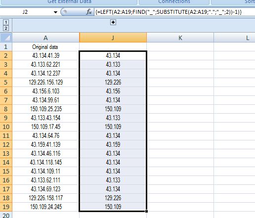
Let rngC1 = Evaluate("IF({1},LEFT(" & rngC1.Address & ",FIND(""_"",SUBSTITUTE(" & rngC1.Address & ",""."",""_"",2))-1))")
Let rngC3 = Evaluate("IF({1},LEFT(" & rngC3.Address & ",FIND(""_"",SUBSTITUTE(" & rngC3.Address & ",""."",""_"",3))-1))")
Application.Wait (Now() + TimeValue("00:00:01"))
Rem 3 Consolidated lists in Dictionary
'3a) make Dics
Dim DicIP2 As Object, DicIP3 As Object
Set DicIP2 = CreateObject("Scripting.Dictionary"): Set DicIP3 = CreateObject("Scripting.Dictionary")
'3b) fill them
Dim rngC1234 As Range: Set rngC1234 = WsSts.Cells(1, NxtClm).Resize(Lra, 4) ' The full 4 column data range, (including title/ comment lines at the top)
Dim arrIn() As Variant: Let arrIn() = rngC1234.Value2
Dim Cnt As Long
For Cnt = 4 To Lra
'3b)(i) The one with first two number groups ( Network Part )
If Not DicIP2.Exists("_" & arrIn(Cnt, 1) & "_") Then '
' Here the Key/Item s pair are made for the first time if this Key dos not exist
DicIP2.Add Key:="_" & arrIn(Cnt, 1) & "_", Item:=arrIn(Cnt, 2) ' The Key is the IP address (part of), the Item is the times it was used
Else ' Else here we Add the infomation of times used if the Key already exists.
' referring to the Item with this key value change its value to what it was added to the value in this next row
Let DicIP2("_" & arrIn(Cnt, 1) & "_") = DicIP2("_" & arrIn(Cnt, 1) & "_") + arrIn(Cnt, 2)
End If
'3b)(ii) The one with first three number groups
If Not DicIP3.Exists("_" & arrIn(Cnt, 3) & "_") Then '
' Here the Key/Item s pair are made for the first time if this Key dos not exist
DicIP3.Add Key:="_" & arrIn(Cnt, 3) & "_", Item:=arrIn(Cnt, 4) ' The Key is the IP address (part of), the Item is the times it was used
Else ' Else here we Add the infomation of times used if the Key already exists.
' referring to the Item with this key value change its value to what it was added to the value in this next row
Let DicIP3("_" & arrIn(Cnt, 3) & "_") = DicIP3("_" & arrIn(Cnt, 3) & "_") + arrIn(Cnt, 4)
End If
Next Cnt
Application.Wait (Now() + TimeValue("00:00:01"))
Rem 4 Output arrays
'4a Output array
'4a(i) The one with first two number groups ( Network Part )
Dim Keys2() As Variant, Itms2() As Variant
Let Keys2() = DicIP2.keys(): Itms2() = DicIP2.items()
Dim arrOut2() As Variant: ReDim arrOut2(0 To UBound(Keys2()), 1 To 2)
For Cnt = 0 To UBound(Keys2())
Let arrOut2(Cnt, 1) = Keys2(Cnt): arrOut2(Cnt, 2) = Itms2(Cnt)
Next Cnt
Application.Wait (Now() + TimeValue("00:00:01"))
'4a(ii) The one with first three number groups
Dim Keys3() As Variant, Itms3() As Variant
Let Keys3() = DicIP3.keys(): Itms3() = DicIP3.items()
Dim arrOut3() As Variant: ReDim arrOut3(0 To UBound(Keys3()), 1 To 2)
For Cnt = 0 To UBound(Keys3())
Let arrOut3(Cnt, 1) = Keys3(Cnt): arrOut3(Cnt, 2) = Itms3(Cnt)
Next Cnt
Application.Wait (Now() + TimeValue("00:00:01"))
Rem 5 Outputs
'5a Output ranges
'5a(i) The one with first two number groups ( Network Part )
Dim rngOut12 As Range: Set rngOut12 = WsSts.Cells.Item(4, NxtClm).Resize(UBound(Keys2()) + 1, 2)
'5a(ii) The one with first three number groups
Dim rngOut34 As Range: Set rngOut34 = WsSts.Cells.Item(4, NxtClm + 2).Resize(UBound(Keys3()) + 1, 2)
'5b 0utputs
rngC1234.Offset(3, 0).Resize(Lra - 3, 4).ClearContents
Let rngOut12 = arrOut2()
Let rngOut34 = arrOut3()
Application.Wait (Now() + TimeValue("00:00:01"))
Rem 6 Sort of
rngOut12.Sort Key1:=rngOut12.Columns(2), order1:=xlDescending
rngOut34.Sort Key1:=rngOut34.Columns(2), order1:=xlDescending
Application.Wait (Now() + TimeValue("00:00:01"))
Rem 7 Some stats
Dim Sum2 As Long: Let Sum2 = Application.WorksheetFunction.Sum(rngOut12.Columns(2))
Let rngOut12.Offset(rngOut12.Rows.Count, 1).Resize(1, 1) = Sum2
Let arrOut2() = rngOut12.Value2
For Cnt = 1 To UBound(arrOut2(), 1)
Let arrOut2(Cnt, 2) = arrOut2(Cnt, 2) & " " & Application.WorksheetFunction.Round((arrOut2(Cnt, 2) / Sum2) * 100, 1) & "%"
Next Cnt
Let rngOut12 = arrOut2()
Application.Wait (Now() + TimeValue("00:00:01"))
Dim Sum3 As Long: Let Sum3 = Application.WorksheetFunction.Sum(rngOut34.Columns(2))
Let rngOut34.Offset(rngOut34.Rows.Count, 1).Resize(1, 1) = Sum3
Let arrOut3() = rngOut34.Value2
For Cnt = 1 To UBound(arrOut3(), 1)
Let arrOut3(Cnt, 2) = arrOut3(Cnt, 2) & " " & Application.WorksheetFunction.Round((arrOut3(Cnt, 2) / Sum3) * 100, 1) & "%"
Next Cnt
Let rngOut34 = arrOut3()
'Application.Wait (Now() + TimeValue("00:00:01"))
End Sub


 Reply With Quote
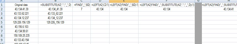
.jpg)


Bookmarks