Appendix Thread. App Index Rws() Clms() Majic code line Codings for other Threads, Tables etc.)

[DocAElstein]

We note a slight difference in order presented in the final results for the level 4s,
https://excelfox.com/forum/showthrea...ll=1#post19943
https://bit.ly/3LpFarN
, when compared with results from the other solutions so far given
https://excelfox.com/forum/showthrea...ll=1#post19944
https://bit.ly/3L5bLBV

- This sort of difference is commonly seen when comparing explorer / recursioning type solutions with simpler looping ones which build up the results one line after the other - recursioning type solutions go up and down the explorer tree view structure thingy and so often order the final results a bit differently.






_____ Workbook: report.xls ( Using Excel 2007 32 bit )

Row\Col	I	J	K	L	M	AE	AF	AG	AH	AI
1	REQUIRE					DATA
2	DIVISION	LEVEL_NO	POSITION	empno	code	DIVISION	LEVEL_NO	POSITION	empno	code
3	XX	1	OZ00301	E1	LL81	XX	1	OZ00301	E1	LL81
4	XX	2	LR0201	E2	LL82	XX	2	LR0201	E2	LL82
5	XX	3	LA0101	E3	LL83	XX	3	LA0101	E3	LL83
6	XX	4	XX0101	E11	LL91	XX	4	XX0101	E11	LL91
7	XX	4	XX0102	E12	LL92	XX	4	XX0102	E12	LL92
8	XX	4	XX0103	E13	LL93	XX	4	XX0103	E13	LL93
9	XX	4	XX0104	E14	LL94	XX	4	XX0104	E14	LL94
10	XX	3	LA0201	E4	LL84	XX	3	LA0201	E4	LL84
11	XX	4	XX0501	E17	LL97	XX	4	XX0502	E6	LL86
12	XX	4	XX0502	E6	LL86	XX	4	XX0601	E7	LL87
13	XX	4	XX0601	E7	LL87	XX	4	XX1901	E8	LL88
14	XX	4	XX1901	E8	LL88	XX	4	XX2101	E9	LL89
15	XX	4	XX2101	E9	LL89	XX	4	XX0501	E17	LL97
16	XX	3	LA0701	E5	LL85	XX	3	LA0701	E5	LL85
17	XX	4	XX0201	E15	LL95	XX	4	XX2201	E10	LL90
18	XX	4	XX0301	E16	LL96	XX	4	XX0201	E15	LL95
19	XX	4	XX2201	E10	LL90	XX	4	XX0301	E16	LL96

Worksheet: Sheet1

[DocAElstein]

Some notes for this forum post https://eileenslounge.com/viewtopic....328185#p328185

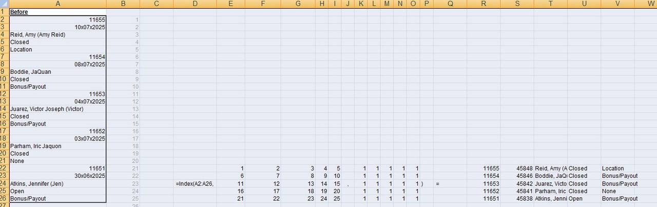
We got this sort of thing in a single column list
Before
11655
10x07x2025
Reid, Amy (Amy Reid)
Closed
Location
11654
08x07x2025
Boddie, JaQuan
Closed
Bonus/Payout
11653
04x07x2025
Juarez, Victor Joseph (Victor)
Closed
Bonus/Payout
11652
03x07x2025
Parham, Iric Jaquon
Closed
None
11651
30x06x2025
Atkins, Jennifer (Jen)
Open
Bonus/Payout
_____ Workbook: TransposeBeautifully.xls ( Using Excel 2007 32 bit )

Row\Col	A
1	Before
2	11655
3	10x07x2025
4	Reid, Amy (Amy Reid)
5	Closed
6	Location
7	11654
8	08x07x2025
9	Boddie, JaQuan
10	Closed
11	Bonus/Payout
12	11653
13	04x07x2025
14	Juarez, Victor Joseph (Victor)
15	Closed
16	Bonus/Payout
17	11652
18	03x07x2025
19	Parham, Iric Jaquon
20	Closed
21	None
22	11651
23	30x06x2025
24	Atkins, Jennifer (Jen)
25	Open
26	Bonus/Payout

Worksheet: Sheet12

We want this sort of thing
_____ Workbook: TransposeBeautifully.xls ( Using Excel 2007 32 bit )

Row\Col	C	D	E	F	G
2	11655	10x07x2025	Reid, Amy (Amy Reid)	Closed	Location
3	11654	08x07x2025	Boddie, JaQuan	Closed	Bonus/Payout
4	11653	04x07x2025	Juarez, Victor Joseph (Victor)	Closed	Bonus/Payout
5	11652	03x07x2025	Parham, Iric Jaquon	Closed	None
6	11651	30x06x2025	Atkins, Jennifer (Jen)	Open	Bonus/Payout

Worksheet: Sheet12

This is a fairly simple and common one that I have done a few times with the
arrOut() = App.Index (arrIn(), Rws(), Clms())
idea

The key to getting the result is to look at what set of array type x,y coordinate pairs are applied to the list to get the required output. It is probably a lot easier to say that in a pic
https://i.postimg.cc/qB6tXScV/arr-Ou...dsheet-pic.jpg



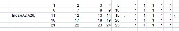
https://i.postimg.cc/J7bv94M1/Index-formula-pic.jpg




Now Excel generally does its "array" things in a convention of columns left to right, then next row, go back to left, then columns left to right, then next row, go back to left, then columns left to right, then next row, go back to left , then ….. etc.
The output comes out in the same locational type way.
In other words our output is going to be in the row,coordinate pairs of like
1,1 2,1,3,1 …. etc
6,1 7,1 8,1 ….etc
….. etc
If you apply those ordinates to our input range/array/single column list, then you can see it will get us the desired output.


So we need to get those two arrays
In an example like this, where a single row or single column is in the input, then we have a convenient characteristic in Excel allowing us to approximately half the work for us to do: It is to do with a bit of theory I call Excel VBA Interception and Implicit Intersection . That is a bit involved, but for us here, it basically means that if I replace that second array with just 1, then Excel in its calculations uses a full array of 1s, where the size is that of the first array. Which in end effect is that second array as shown.
So we can forget about the second array, and our job is to get the first one.

There are 2 things , ( well, 3 depending on your point of view, – 2 Excel Functions and a convenient characteristic ) helpful to know about and use for this:
_ We have these sort of things in Excel
ROW(1:3) =
1;
2;
3
COLUMN(A:B)=
1, 2
So they are very convenient for getting us a "vertical" or "horizontal" array of numbers

The convenient characteristic is similar to the one mentioned before. Once again it come out of the Excel VBA Interception and Implicit Intersection theory idea, and it is that if I have a single row or a single column, and attempt to do some calculation, such as, for example
ROW(1:3) x COLUMN(A:B)
, then effectively the "missing" values needed will be taken as a duplicate of the row or column. In other words, using the same example, I wont be doing this

1
2    X   1  2
3

, but rather effectively I will be doing this

1  1       1  2
2  2   X   1  2
3  3       1  2

, in the coordinate pair type way as discussed already.
So in that example I will end up with an array like

1  2
2  4
3  6

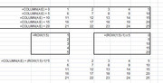
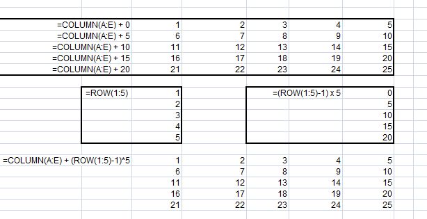
So basically messing around with the spreadsheet functions ROW() and COLUMN() and maybe a bit of maths will usually get us the final array we want

This is the first solution I came up with that gets the array I want is
=COLUMN(A:E) + (ROW(1:5)-1)*5

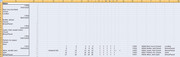
In the uploaded file you can see some of the workings to get that:
https://i.postimg.cc/JhWFzf1N/COLUMN...W-1-5-1-x5.jpg




Here some coding with a few more ' explanations

Sub TransformBeautifully() ' https://eileenslounge.com/viewtopic.php?p=328185#p328185
Dim WsMe As Worksheet: Set WsMe = ActiveSheet
Dim Lr As Long, En ' To make the solution dynamically beautiful
 Let Lr = WsMe.Range("A" & WsMe.Rows.Count & "").End(xlUp).Row
' The Row number needed for final output
 Let En = (Lr - 1) / 5 ' This assumes the start is row 2
' or
 Let Lr = WsMe.Range("A" & WsMe.Rows.Count & "").End(xlUp).Row
 Let En = Lr \ 5  '  This allows for the start from any of the first few rows

' We are doing this sort of thing  Index(Array,{Rows()},1)
' {Rows()} needs to be an array like this sort of form:
'                            1   2   3   4   5
'                            6   7   8   9   10
'                            11  12  13  14  15
'                            16  17  18  19  20
'                            21  22  23  24  25
'
' we can usually get arrays like that by messing with the spreadsheet functions  ROW()  and  COLUMN()  and  a bit of maths
Dim Rws() As Variant
 Let Rws() = WsMe.Evaluate("COLUMN(A:E) + (ROW(1:5)-1)*5") ' we use the  Evaluate("")  to use spreadsheet things in VBA, which is useful here as we do not have similar functions to  ROW()  and  COLUMN()
 Let Rws() = WsMe.Evaluate("COLUMN(A:E) + (ROW(1:" & En & ")-1)*5") ' we use the  Evaluate("")  to use spreadsheet things in VBA, which is useful here as we do not have similar functions to  ROW()  and  COLUMN()
' , but we can use some workshet functions directly in VBA, which at a geuss might be more efficient than using  Evaluate("")
Dim arrOut() As Variant
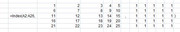
 Let arrOut() = Application.Index(WsMe.Range("A2:A26"), Rws(), 1)
 
 Let WsMe.Range("C2").Resize(En, 5) = arrOut()
 Let WsMe.Range("C2").Resize(En, 5) = Application.Index(WsMe.Range("A2:A26"), Rws(), 1)
 Let WsMe.Range("C2").Resize(En, 5) = Application.Index(WsMe.Range("A2:A26"), WsMe.Evaluate("COLUMN(A:E) + (ROW(1:" & En & ")-1)*5"), 1)
 Let WsMe.Range("C2").Resize(En, 5) = Application.Index(WsMe.Range("A2:A26"), WsMe.Evaluate("COLUMN(A:E) + (ROW(1:" & Lr \ 5 & ")-1)*5"), 1)
 Let WsMe.Range("C2").Resize(En, 5) = Application.Index(WsMe.Range("A2:A26"), WsMe.Evaluate("COLUMN(A:E) + (ROW(1:" & WsMe.Range("A" & WsMe.Rows.Count & "").End(xlUp).Row \ 5 & ")-1)*5"), 1)
 Let WsMe.Range("C2").Resize(Lr \ 5, 5) = Application.Index(WsMe.Range("A2:A26"), WsMe.Evaluate("COLUMN(A:E) + (ROW(1:" & WsMe.Range("A" & WsMe.Rows.Count & "").End(xlUp).Row \ 5 & ")-1)*5"), 1)
 Let WsMe.Range("C2").Resize(WsMe.Range("A" & WsMe.Rows.Count & "").End(xlUp).Row \ 5, 5) = Application.Index(WsMe.Range("A2:A26"), WsMe.Evaluate("COLUMN(A:E) + (ROW(1:" & WsMe.Range("A" & WsMe.Rows.Count & "").End(xlUp).Row \ 5 & ")-1)*5"), 1)
 Let WsMe.Range("C2").Resize(WsMe.Range("A" & WsMe.Rows.Count & "").End(xlUp).Row \ 5, 5) = Application.Index(WsMe.Range("A2:A" & WsMe.Range("A" & WsMe.Rows.Count & "").End(xlUp).Row & ""), WsMe.Evaluate("COLUMN(A:E) + (ROW(1:" & WsMe.Range("A" & WsMe.Rows.Count & "").End(xlUp).Row \ 5 & ")-1)*5"), 1)
 
 Range("C2").Resize(Range("A" & Rows.Count).End(xlUp).Row \ 5, 5) = Application.Index(Range("A2:A" & Range("A" & Rows.Count & "").End(xlUp).Row), Evaluate("COLUMN(A:E) + (ROW(1:" & Range("A" & Rows.Count).End(xlUp).Row \ 5 & ")-1)*5"), 1)

End Sub