We are almost there.
We need to make some construction using that WorkRange.Address within VBA that allows it to be used within the main formula string: We cannot just insert WorkRange.Address any more as we cannot just insert WorkRange, as it will take WorkRange.Address as just that actual text, as if we had given excel some text, like
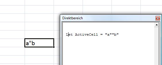
Let ActiveCell = "WorkRange.Address" ___ 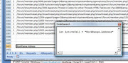
, but we don't want that, we want the short text notation used in an Excel spreadsheet for a range, (that of the cell in the Excel spreadsheet column letter and row number format), that is returned from WorkRange.Address when it is used in VBA coding.
The VBA coding syntax for doing that sort of thing is to insert it into the main formula string at the appropriate position in a special way like this
_______________ " & WorkRange.Address & "
What that does, is do the VBA business on WorkRange.Address and then stick the result into the literal text
, pseudo like, if , for example, WorkRange was the second cell in a spreadsheet, ( Set WorkRange = Range("B1") ) then:
" & WorkRange.Address & " will be turned by VBA into $B$1 , and that $B$1 will be inserted into the text.
We are using it in a formula, but the idea is easier to see in a simple text, thus
Code:
Sub TextIn()
Dim Rng As Range
Set Rng = Range("A1")
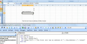
Let Range("D10") = "The first cell has an address of " & Rng.Address & ", honest"
End Sub
Rub that macro and then In the cell, D10 you will see
The first cell has an address of $A$1, honest
In this post we will now do some examples of how to put the basic formula into a cell. Some will be relevant to this Thread, some won't necessarily, - at the end of the day we are Human here and are not so keen to encourage the robots to take over with their well ordered cold logic!
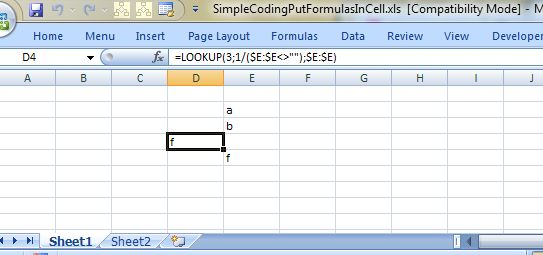
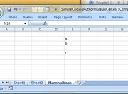
From now on I will use this simple test range, which is in both worksheets in the uploaded file. ( the letter f in cell E5 is the last filled cell in column E)
https://i.postimg.cc/Kz4bFvvc/Simple-test-range.jpg 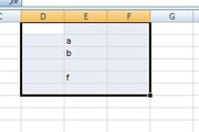
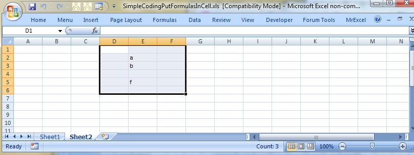
_____ Workbook: SimpleCodingPutFormulasInCell.xls ( Using Excel 2007 32 bit )
| Row\Col |
E |
|---|
| 1 |
|
| 2 |
a |
| 3 |
b |
| 4 |
|
| 5 |
f |
| 6 |
|
Often, or at least initially, I will tend to put the formula somewhere to the left of the range, for no particular reason other than a guess that it could bee convenient there. Of course, if I am passing a work range, then that will determine where things are relatively speaking.
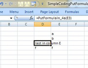
Simplest Codings Put formula in
I assume here that I want my formula in column D, and I have selected the cell in column D that I want the formula in.
Here are three coding offerings
Code:
Sub PutFormulaIn_1()
 Let ActiveCell = "=LOOKUP(3,1/(" & ActiveCell.Offset(0, 1).EntireColumn.Address & "<>"""")," & ActiveCell.Offset(0, 1).EntireColumn.Address & ")"
End Sub

Sub PutFormulaIn_2a()
Call PutFormulaIn_2b(ActiveCell.Offset(0, 1).EntireColumn)
End Sub
Sub PutFormulaIn_2b(ByVal WorkRange As Range)
 Let ActiveCell = "=LOOKUP(3,1/(" & WorkRange.Address & "<>"""")," & WorkRange.Address & ")"
End Sub

Sub PutFormulaIn_3a()
Call PutFormulaIn_3b(ActiveCell.Offset(0, 1).EntireColumn)
End Sub
Function PutFormulaIn_3b(ByVal WorkRange As Range)
 Let ActiveCell = "=LOOKUP(3,1/(" & WorkRange.Address & "<>"""")," & WorkRange.Address & ")"
End Function
(The coding is also in the uploaded file, SimpleCodingPutFormulasInCell.xls )
Run any of those codings, ( by running either of these:
Sub PutFormulaIn_1()
Sub PutFormulaIn_2a()
Sub PutFormulaIn_3a() __
), and the result will be the same:
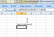
In the selected cell, if it is in column D you will see f
In the formula bar you will see =LOOKUP(3,1/($E:$E<>""),$E:$E)
https://i.postimg.cc/BnZzPSR3/Result...ist-Coding.jpg
Strictly speaking, none of those solutions is a UDF solution.
The last function could be considered a UDF, if I called it from the spreadsheet by typing in any cell something like
=PutFormulaIn_3b(E:E)
If you try doing it just like that it will not work. That is where the typical answers come from, those answers of like ….
…. A UDF cannot add a formula to a cell. …..
In the next post I will show how that can be done. But before that I will throw in a solution of a different sort, just in case it might be worth considering….
Simple alternative way to do it Event Coding
This solution does not really fit in to this Thread. But we are not prejudice here at excel fox.
Event Coding
VBA can be thought very approximately as the coding that actually makes Excel or Microsoft Office work. Very graciously Microsoft let us tap into it, and so we can do an amazing number of things.
(Using Microsoft Office without the VBA you already have, can be compared with having some all purpose vehicle parked outside your door, that can do just about everything that any vehicle can and much more like flying to Mars, submerging to the centre of the earth, digging out a trench to make a river to save a Forest for younger generations etc., etc., but you just use it once a week for the same short journey to go to the local shops )
Microsoft do not let us do everything, understandably perhaps, or else we would make everything ourselves, or more likely make a mess.
When things happen, for example, a cell value gets changed, various things happen, a chain of events occur, as it were. We can tap into those as well.
We will do that in worksheet, Sheet2
We go to the second worksheet, Sheet2, right click on the Sheet2 tab at the bottom, select View Code , that gets us the VB Editor we might be familiar with, but the biggest empty window showing is a special code module belonging to the worksheet. There is one such code module for each worksheet.
https://i.postimg.cc/F15RRvcj/Mess-a...eet-Change.jpg
Now mess around selecting things from the two drop downs you see at the top of the worksheet code module until you get the Worksheet_Change sub routine showing
It is empty initially. It is part of the chain events that happen when something is changed in a worksheet. Microsoft do not want to show us all that goes on, but we can see this sub routine that is always done, or rather run, even though it does nothing as it is empty. But we can add coding to it, so that something else is done when there is a change in the worksheet.
The Target variable is given to us and filled with the range object of what was changed. So that is handy, me thinks…..
How about this:
I will write a bit of coding to put in the empty routine, that checks what range got changed. If it was a single cell, and say, a small z was typed in, then I will put the formula in that cell, the formula that gives me the last value in the column to the right of that cell
Here is the coding
Code:
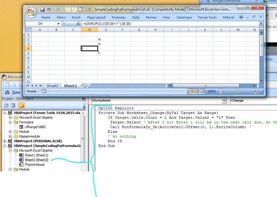
Private Sub Worksheet_Change(ByVal Target As Range)
    If Target.Cells.Count = 1 And Target.Value2 = "z" Then
     Target.Select ' After I hit Enter I will be in the next cell down, so this puts me back in the cell I typed  z  in
     Call PutFormulaIn_3b(ActiveCell.Offset(0, 1).EntireColumn) '
    Else
    ' do nothing
    End If
End Sub
The coding is also in the uploaded file, SimpleCodingPutFormulasInCell.xls
So just to recap, clarify what you do and what goes on in Sheet2:
Select a cell (in Sheet2), to the left of the column you want to get the last value of, for example D4.
Type a small z in it, and hit Enter 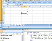
The formula we want then gets put in that cell, ( the z is overwritten with the formula )
For convenience I use the function PutFormulaIn_3b . I could just as well have put all the coding in , or indeed used any of the other routines .
Code:
Private Sub Worksheet_Change(ByVal Target As Range)
    If Target.Cells.Count = 1 And Target.Value2 = "z" Then
     Target.Select ' After I hit Enter I will be in the next cell down, so this puts me back in the cell I typed  z  in
'     Call PutFormulaIn_3b(ActiveCell.Offset(0, 1).EntireColumn) '
'     Call PutFormulaIn_1
'     Call PutFormulaIn_2a
'     Call PutFormulaIn_2b(ActiveCell.Offset(0, 1).EntireColumn)
     Call PutFormulaIn_3a
    Else
    ' do nothing
    End If
End Sub


 Reply With Quote
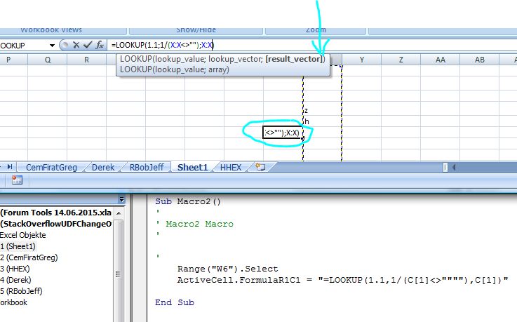


Bookmarks